|
Introduction
|
A Geiger-Mueller (GM) tube is a gas-filled radiation detector. It commonly takes the form of a cylindrical outer shell (cathode) and the sealed gas-filled space with a thin central wire (the anode) held at ~ 1 KV positive voltage with respect to the cathode. The fill gas is generally argon at a pressure of less than 0.l atm plus a small quantity of a quenching vapor (whose function is described below).
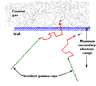
If a gamma - ray interacts with the GM tube (primarily with the wall by either the Photoelectric Effect or Compton scattering) it will produce an energetic electron that may pass through the interior of the tube.
Figure 1. The principal mechanism by which gas-filled counters are sensitive to gamma- rays involves ejection of electrons from the counter wall. Only those interactions that occur within an electron range of the wall's inner surface can result in an output pulse.
Ionization along the path of the primary electron results in low energy electrons that will be accelerated towards the center wire by the strong electric field. Collisions with the fill gas produce excited states (~11.6eV) that decay with the emission of a UV photon and electron-ion pairs (~26.4 eV for argon). The new electrons, plus the original, are accelerated to produce a cascade of ionization called "gas multiplication" or a Townsend avalanche. The multiplication factor for one avalanche is typically 106 to 108. Photons emitted can either directly ionize gas molecules or strike the cathode wall, liberating additional electrons that quickly produce additional avalanches at sites removed from the original. Thus a dense sheath of ionization propagates along the central wire in both directions, away from the region of initial excitation, producing what is termed a Geiger-Mueller discharge.
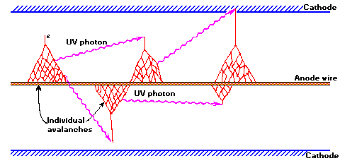
Figure 2. The mechanism by which additional avalanches are triggered in a Geiger-Mueller discharge.
The intense electric field near the anode collects the electrons to the anode and repels the positive ions. Electron mobility is ~ 104 m/s or 104 times higher than that for positive ions. Electrons are collected (by the anode) within a few µs, while the sheath of massive positive ions (space charge) surrounding the center wire are collected within a few "ms" by the cathode.
The temporary presence of a positive space charge surrounding the central anode terminates production of additional avalanches by reducing the field gradient near the center wire below the avalanche threshold. If ions reach the cathode with sufficient energy they can liberate new electrons, starting the process all over again, producing an endless continuous discharge that would render the detector useless. An early method for preventing this used external circuitry to "quench" the tube, but the introduction of organic or halogen vapors is now preferred. The complex molecule of the quenching vapor is selected to have a lower ionization potential ( < 10 eV) than that of the fill gas (26.4 eV) and is present with a concentration fo about 5 ÷10 %. This kind of gas, prevents multiple pulsing through the mechanism of charge transfer collision. Infact the positive ions formed by the incident radiation are mostly of he primary component (for example Argon), and they subsequently make many collisions with neutral gas molecules as they drift toward the cathode. Some of this collisions will be withmolecules of the quebch gas and, because of the difference in ionization energies, there will be a tendency to transfer the positive charge to the quench gas molecule. The original positive ion is thas neutralized by transfer of an electron, and a positive ion of the quench gas begins to drift in its place.Now if the concentration of the quenching gas is sufficiently high, these charge transfer collisions assure that all the ions that eventually arrive at the cathode will be those of the quench gas. Also when they are neutralized, the excess energy may now go into disassociation of the more complex molecules in preference to liberating a free electron from the cathod surface. It's obvious that with the proper choice of quenching gas, the probability of disassociation can be made much larger than that of electron emission and therfore no additional avalanches are formed withing the tube. Organic quench vapors, such as alcohols, are permanently altered by this process, limiting tube life to ~ 109 counts. Halogen quench vapors (like chlorine or bromine for example) dissociate in a reversible manner later recombining for an essentially infinite life.
The sheath of positive ions (space charge) close to the anode reduces the intense electric field sufficiently that approaching electrons do not gain sufficient energy to start new avalanches. The detector is then inoperative (dead) for the time required for the ion sheath to migrate outward far enough for the field gradient to recover above the avalanche threshold. The Dead Time of a Geiger tube is defined as the period between the initial pulse and the time at witch a second Geiger discharge, regardless of its size, can be developed. In most Geiger tubes, this time is of the order of 50 ÷ 100 µs.
The GM tube output is a charge pulse whose amplitude is independent of the energy of the detected radiation. The only amplitude information that it can provide is that the energy of the detected radiation was sufficient to produce electrons energetic enough to penetrate to the sensitive region of the tube. The quantity of charge produced is directly proportional to the "over voltage", i.e., the difference between the GM threshold voltage at which a GM discharge will first occur, and the higher normal operating voltage. The output signal will be directly proportional to the charge (108 - 1010 ion-pairs), and inversely proportional to the circuit capacitance (GM tube capacitance + the connecting cable capacitance + the input capacitance of the electronic system). The normal signal is of the order of volts.
It is assumed that you are familiar with statistics and the definitions for sample and population means, variances, and probability distribution.
The definitions of these symbols are:
Sample Mean: ![]()
Sample Variance: ![]()
(Note the N - 1 in the definition of s2 makes s2 a correct estimator of sigma2.)
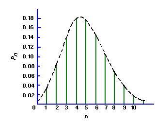
Under the conditions that are thought to apply to all radioactive decays (i.e., all the nuclei are identical, independent, and each has a definite and constant probability of decay in a unit time interval), one can derive a distribution function P(x) that is the probability of observing x counts in one observation period.
The distribution of the values x about the true average µ is called the Poisson distribution and has the form:
 (2)
(2)
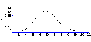
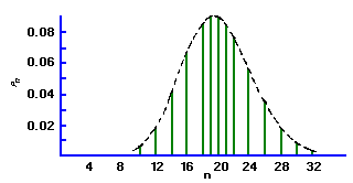
If the mean of a Poisson distribution becomes ~20, the distribution becomes symmetrical, assuming the characteristics of a Normal, or bell-shaped Gaussian distribution. This displays the characteristic that 68% of the total area of the distribution lies within ± sigma of the mean. For a Poisson distribution sigma=sqrt(µ) , so that a counting measurement is 68% likely to be within ± sigma of the true population mean µ Since x is probably close to µ, we may take sigma = sqrt(x), and say that a single measurement is 68% likely to be within ± sqrt(x) of the true mean. Similarly the values for ± 2 sigma and ± 3 sigma are 95% and 99.7%, respectively. When plotting experimental results, it is customary to include error bars of length sigma1 on each point xi.
Often a desired value is a function of several measured values each of which has finite statistical uncertainties. If a value Z = f (X,Y) is a function of independent random variables X and Y, there will be a certain spread in Z associated with spreads in the values of X and Y. By using probability theory it is not difficult to derive the following general formula:
![]()
which relates the expected uncertainty in a calculation of Z to the corresponding uncertainties, sigmax and sigmay , of X and Y. Both the random variables X and Y must have a normal distribution, with the uncertainties in both X and Y small enough so that the differentials accurately describe the variations in Z. Note also that Poisson random variables are nearly normal when m > 20, so that this formula usually will hold quite well.
Characteristics of the GM counter
Put a radioactive source below the GM tube. Put the counter in a counting mode and raise the voltage until counts are observed. Note the shape of the pulse and what happens as the voltage on the GM tube is increased. Do not exceed 900 volts at this time. What is the minimum voltage pulse necessary to activate the counter? After properly triggering the scope, sketch a picture of the pulse shape.
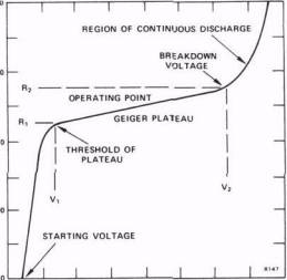
Every GM tube has a characteristic response of counting rate versus voltage applied to the tube. A curve representing the variation of counting rate with voltage is called a plateau curve because of its appearance. The plateau curve of every tube that is to be used for the first time should be drawn in order to determine the optimum operating voltage. Find the plateau curve for your tube using the procedure outlined below.
A. Check to see that the high voltage as indicated by the meter on the instrument is at its minimum value.
B. Insert a radioactive source into one of the shelves of the counting chamber. Choose shelf and counting time such that you have at least 1000 counts in the plateau region.
C. Turn on the count switch and slowly increase the high voltage until counts just begin to be recorded by the scaler. The voltage at which counts just begin is called the "starting voltage" of the tube.
D. Beginning at the nearest 20 volt mark above the starting voltage, take one-minute (longer time if counting rate is too low) counts every 40 volts until a voltage is reached where a rapid increase in counts is observed. Reset scaler to zero before each count. Tabulate counts versus voltage.
E. Plot the data of (D). A plateau should be observed in the curve.
The optimum operating voltage will be about the middle of the plateau, usually some 150 to 200 volts above the knee of the curve. Set the high voltage to this point and record. The slope S of the plateau of a GM tube serves as a figure of merit for the tube.
The slope is defined to be the percent change in count rate per 100 volts change in applied voltage in the plateau region. A slope of greater than 10% indicates that the tube should no longer be used for accurate work.
The slope may be computed using
S (% per 100 V) = 2 (R2 - R1) 10^4 /(R2 + R1) (V2 - V1)
where V2 is the voltage at the high end of plateau, R2 is the count rate at this voltage, V1 is the voltage at the low end of the plateau, and R1 the corresponding rate. In order to compare, obtain a similar plateau curve for an old tube (if available).
Resolving time of the GM counter
There is an interval of time following the production of a pulse in the GM tube during which no other pulse can be recorded. This interval is called the resolving time of the system. If this time is known it can be used to make a correction to the observed count rate to yield the true count rate. The procedure below can give a good estimate of the resolving time.
A. Obtain a resolving time source (a "split source"). This source is split into two parts. Remove one half of the source and set it aside.
B. Place the carrier containing one part on the second shelf of the counting chamber and make a trial count of 1 minute duration. Get the maximum count rate you can. Hopefully this should be more than 20,000 counts per minute, but if not use what you can get.
C. Make a 3-minute count and record the counts per minute, R1.
D. Put the two parts of the source back together, taking care not to disturb the position of the first part. Make a 3-minute count of the combined parts and record as Rc.
E. Remove the part initially counted and make a 3 minute count on the second part. Record as R2 (counts per minute). F. Calculate the resolving time of the GM system using the relation:
t = (R1 + R2 - Rc)/ (2*R1*R2)
Convert the time thus found to microseconds/count and record. The resolving time t may be used to correct an observed count rate using the expression:
R = r/(1-r*t)
where:
r = Observed count rate
R = True count rate
|
Element |
Energy of Radiation |
Half-Life |
|
|
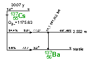
Cesium 137 |
beta - 0.51397 |
30.07 yr |
|
|
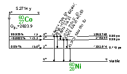
Cobalt 60 |
beta - 0.31786 |
5.2714 yr |
|
|
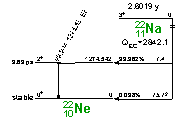
Sodium 22 |
beta + 0.5454 |
2.6019 yr |
|